← all notes

3 Jul 2026 · 14 min read

paytrail: building a payments warehouse

A governed medallion lakehouse over 6.3 million synthetic payments, no fraud model by design. Every figure traces back to its source, and a Databricks benchmark I ran came out 39% faster, for a reason I did not expect.

A compliance analyst checks the day’s settled figure against the ledger before it goes into a report. A product manager reads it to see which payment types are growing.

paytrail is a small version of the warehouse behind a figure like that. It takes about 6.3 million synthetic transactions, moves them through a three-stage pipeline, and produces a daily total that any figure can be traced back to the row it came from. The synthetic data is a deliberate choice (PaySim, a public tool that generates realistic but fake payments), and there is no fraud-detection model anywhere in it, also on purpose. The dataset comes with a fraud flag, and I left it as a column to report rather than a thing to predict. What I wanted to practise is the part that decides whether a reported number matches the raw data it came from: loading it so a repeat never double-counts, removing duplicate records, proving nothing went missing along the way, and keeping sensitive fields away from anyone with no reason to see them.

Bronze, silver, gold

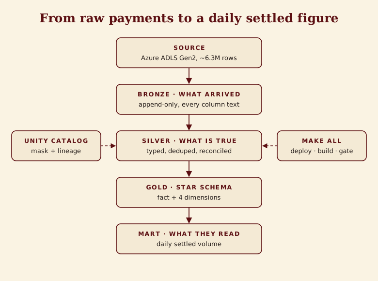
The pipeline has three layers, and this bronze, silver, gold naming is a common pattern for it (the “medallion” architecture). Raw data comes in one side and a finished report comes out the other, and each layer has one job. The reason to split the work this way is that any stage can be re-run on its own, and there is always a faithful copy of the original input to trace a figure back to.

Bronze is what arrived. The source file is read from Azure cloud storage and written into the warehouse exactly as received, with rows only ever added and never edited, and every column stored as plain text so an odd value can never crash the load. Bronze is the anchor: whatever a later figure turns out to be, it can be traced to the bronze row it came from, and the whole pipeline can be rebuilt from here.

Silver is what is true. Here the data is cleaned up: each value is given its proper type so a date reads as a date and an amount as a number, the account identifiers are put in a consistent form, duplicate records are merged, and any row that fails a check is set aside with the reason it failed. This is the layer that turns a faithful copy into figures I am willing to report.

Gold is what the business reads. The cleaned data is reshaped into the layout a reporting tool likes, called a star schema: one central table with a row per transaction, surrounded by smaller tables that describe the accounts, customers, dates, and transaction types involved. That shape keeps the summing-up queries simple. On top of it is one mart, which is just a small table built to answer a single set of questions. Here it contains daily settled volume split by transaction type and customer segment, already added up, so a dashboard can read one table instead of re-combining the big tables every time.

It runs on Databricks, reading its source from Azure cloud storage. The transformations and the data-quality tests are written in dbt, and Unity Catalog governs who can see what and tracks where each figure came from. Every step is a Python script or a dbt model kept in version control, so the whole pipeline is reproducible and nothing runs by hand in a notebook.

Cleaning and reconciling in silver

Silver is where raw records become numbers I would put in a report, so it is where most of the work went. Five things have to be true, and each one prevents a specific way the total could go wrong.

Loading that can safely repeat. A batch of files can be loaded twice, by a job that retried or a manual re-run, and a warehouse that counts the repeat reports too high a total. Each file is tagged with its name, so a file already loaded is skipped before it is read, and running the same load again changes nothing. (The technical word for this is idempotent.)

Removing duplicate records. Two copies of the same payment should count once. Each event is given a fingerprint built from its details, its time-step, type, source and destination accounts, and amount, and if the same fingerprint turns up twice, only one copy is kept.

Handling data that arrives late or out of order. A payment carries two timestamps: when the event happened, and when its row reached the warehouse. A correction can arrive later but describe an earlier event. Silver sorts by when things happened, not by when they arrived, so a late correction is still placed in its correct day, and when the same event turns up more than once the most recently loaded copy wins, so a correction replaces the original.

Setting bad rows aside instead of throwing them away. A row that fails one of six checks, a missing account, an impossible time-step, an unreadable or negative amount, a negative balance, or an unknown account type, is written to a separate quarantine table with the reason it failed. Nothing is silently discarded, and the count of quarantined rows is a health signal in its own right.

Proving nothing was lost. Before I report anything, I want to show that every raw row is accounted for. Each bronze row ends up in exactly one place: set aside in quarantine, kept as clean, or merged into another row as a duplicate. Add those up and the total has to equal the bronze count, and the amounts have to match to the penny. A test checks that on every build, and if it ever fails, the build stops before the number reaches anyone. At the full 6,362,620 rows, the counts tie and the amounts tie to the penny.

There is a catch with clean data. Every row in the PaySim file passes the checks, so the quarantine table stays empty and the duplicate-handling never actually runs on the genuine data. The only way to prove that code works is to feed it faulty rows on purpose. Two small tests do exactly that: one sends a deliberately faulty row for each of the six checks and confirms it is set aside with the right reason, the other sends a duplicate and confirms only the latest copy survives. Clean data cannot test the code that only runs when data is bad.

Of the 51 tests every build runs, 48 are schema and referential-integrity checks (uniqueness, not-null, accepted values, and the six foreign keys from the fact table to its dimensions), one is the reconciliation gate above, and two are the fault-injection unit tests just described.

-- bronze = quarantine + clean_eligible
-- clean_eligible = clean + duplicates_removed
-- every bronze row is quarantined, kept, or removed as a duplicate

row_number() over (
    partition by transaction_id
    order by _load_ts desc, event_ts asc
) as _row_rank

How account data is governed

Governance here means two things working together: who may see a raw account identifier, and where that identifier is allowed to travel.

A masking rule covers the two columns that contain account numbers in the raw layer. The database applies it automatically on every read, so there is no way to slip past it. Whoever has a legitimate reason to see raw account numbers gets the full value, everyone else gets *** and the last four characters, the way the end of a card number is shown on a receipt. The pipeline itself is allowed, because the cleaning step has to read the actual account numbers to standardise them and swap them for safe stand-ins. Everyone and everything else sees only the masked version.

As the data moves into the cleaned layer, each account number is replaced by a SHA-256 token: a stable pseudonym, so the same account always maps to the same key and downstream joins work without the original string. A plain hash is not strong protection for an id like this, an account number is short and structured, so its whole range is small enough to brute-force or look up in a precomputed table. On production data I would use a keyed hash (HMAC, with the key held apart from the data) or a separately-held salt, so the mapping cannot be recovered. What the token buys here is defence in depth: with the column mask on the raw layer, it keeps the literal account number out of every table past silver. The catalogue also records lineage automatically, a map of which table’s data came from which, so any figure in the final report can be traced back through the layers to the raw row it started as.

The *** plus last-four pattern is the same truncation rule applied to a card number under the Payment Card Industry Data Security Standard (PCI-DSS), and it limits who can read personally identifiable information (PII), the data-minimisation principle behind GDPR, the EU’s data-protection law. On synthetic data none of it protects a person, which is the reason to prove the mechanism on data where a mistake costs nothing.

CREATE OR REPLACE FUNCTION paytrail.bronze.mask_account(account STRING)
  RETURNS STRING
  RETURN CASE
    WHEN is_member('paytrail_pii_readers') THEN account
    ELSE CONCAT('***', RIGHT(account, 4))
  END;

One command, and the constraint behind it

The whole pipeline runs from a single command, make all. It sets up the catalogue and permissions, deploys the project to Databricks (the setup is written as code, so it is repeatable), loads the raw data from Azure, runs every model and all 51 data-quality tests, runs a job on the Databricks side, and then runs the benchmark.

The free tier has one limit that shaped the design. It cannot run the transformation and Python steps as part of the Databricks job itself, because that needs a kind of compute the free tier does not include, so the job would fail to start. So the transformations run from my command line instead, and the job on the Databricks side is a single guard query: it checks that the final tables are not empty and that the reconciliation still balances, and it fails the whole run if either is wrong. That guard is simpler than a full pipeline running inside Databricks, and it still stops the run when the data is wrong, which is what I wanted from it.

The benchmark that didn’t do what I set it up to do

The final table feeds a dashboard, the view a product manager would read.

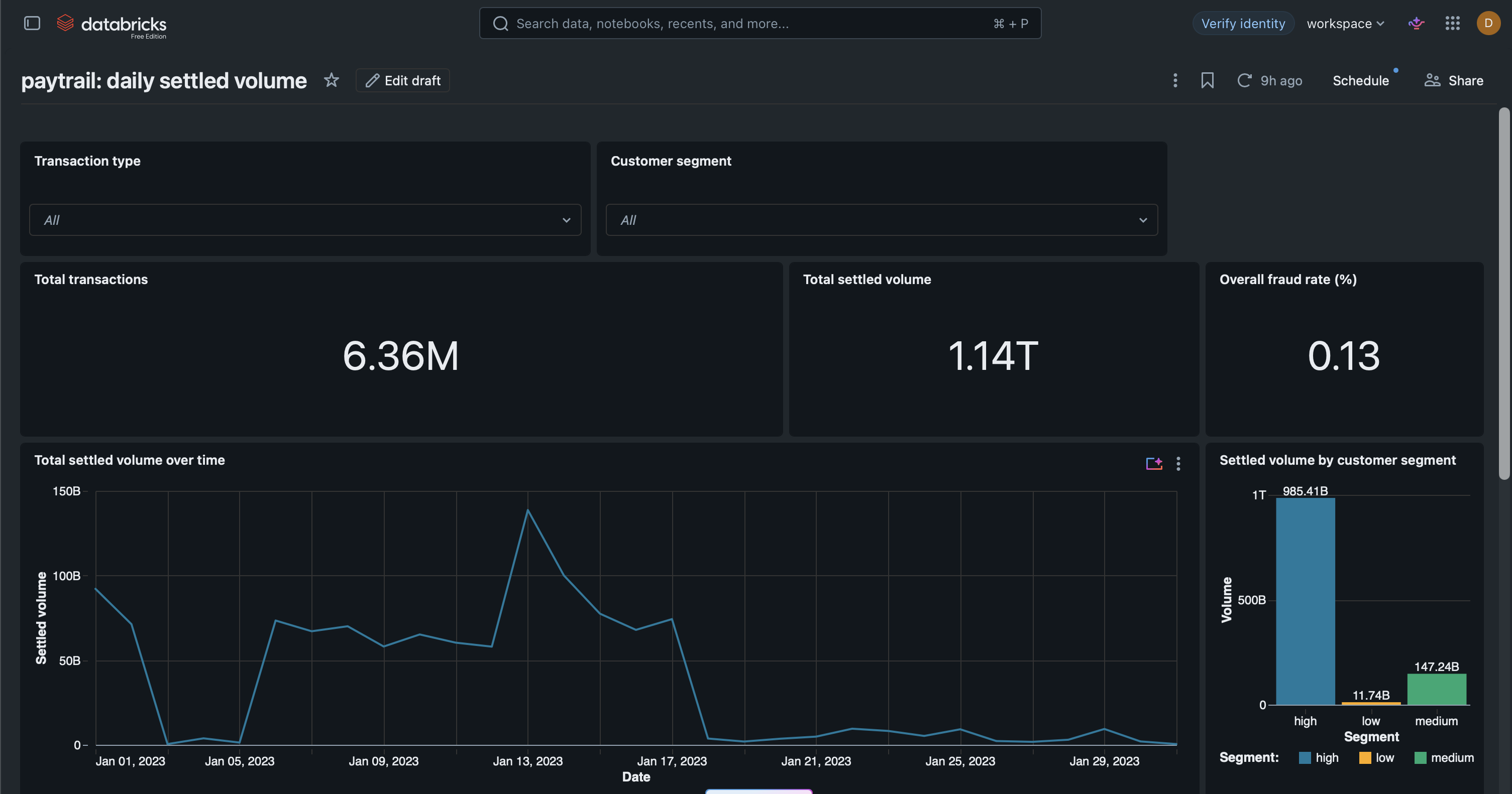
Refreshing that dashboard runs one heavy query: add up every transaction amount by day and by type across a two-week window. I wanted to measure what happens to that query when I change how the data is physically laid out on disk, so I timed it before and after a Databricks command called OPTIMIZE with Z-ordering.

Z-ordering rearranges the stored files so that rows with similar dates and types are grouped into the same files. In principle, a query filtered to two weeks can then skip the files that contain no rows from those weeks, and read less. I deliberately stored the table as 96 small files, ran the two-week query, then ran the OPTIMIZE command and ran the same query again.

The query got faster. The time the server spent on it fell from 1.62 seconds to 0.98, a 39% reduction, and the number of files it had to open fell from 96 to 4.

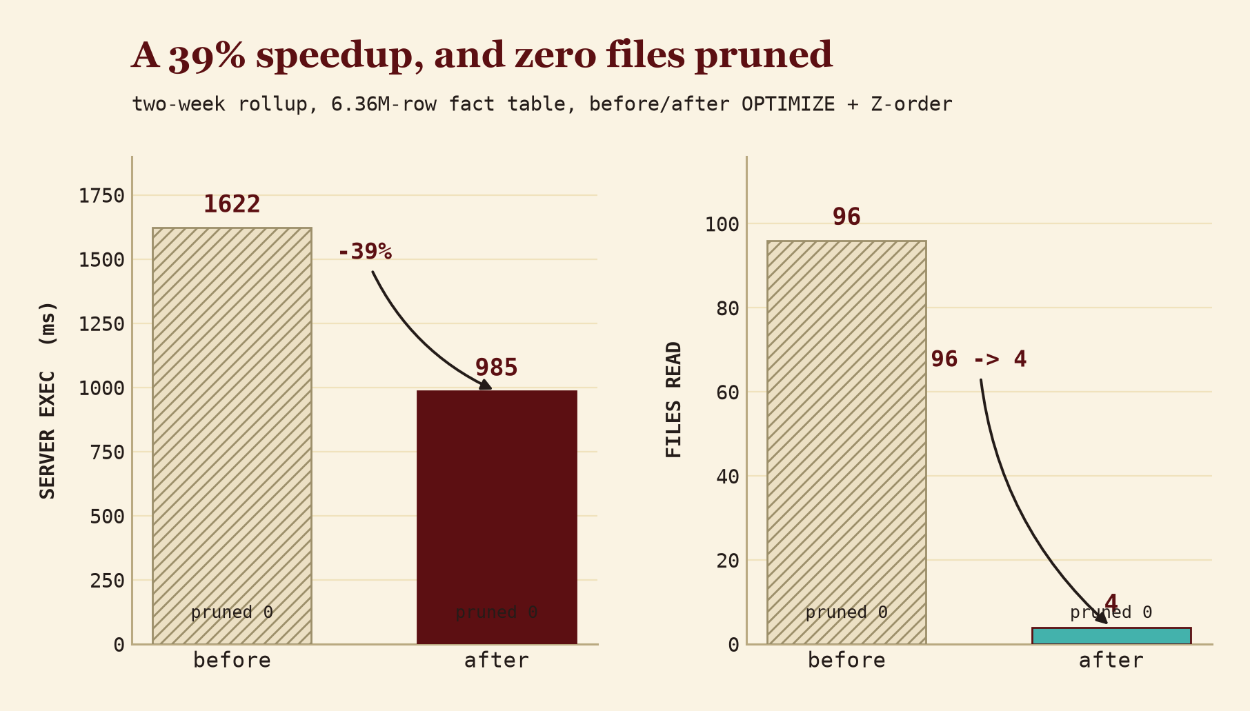
Then I looked at why. Databricks reports, for every query, how many files it skipped. That count was zero both times, before and after Z-ordering, even at the full 6.36 million rows. Nothing was skipped. OPTIMIZE had merged the 96 small files into 4 large ones, each covering about a week, so a two-week filter overlaps all four of them and none can be skipped. The amount of data read barely changed, 30.8 MB before and 27.9 MB after, and the number of rows read was identical at 4,133,856. The same data was simply read from fewer files. So the speedup came from merging small files, opening 4 instead of 96 is cheaper, rather than from the file-skipping I set the benchmark up to show. At this size the whole table fits in four files, so there is nothing to skip.

The stopwatch numbers are shaky, though. The free tier already optimises queries on its own (a feature called Predictive I/O), so the slower case is partly tuned before I even start, and the timings wander from run to run. The numbers I trust are the ones I can point to: how many files were read, how much data, and the server’s own execution time. To actually get file-skipping, the table would need to be big enough that OPTIMIZE leaves many files per week, or organised on disk by date (through partitioning or liquid clustering) so a two-week filter only touches a small slice. That is the change I would make on a production-sized dataset.

The result I can stand behind is narrower than the one I set out to produce: the query got 39% faster, and not one file was skipped to make it happen. Quoting the 39% on its own would let a reader assume the clever file-skipping did the work, when the numbers point to the plainer cause, fewer and larger files.

That is the same habit as the rest of the build: put a number on the table, then be able to say exactly what produced it. It is what lets the compliance analyst file the settlement figure and the product manager act on it without re-checking six million rows, because every row is accounted for across the layers and every figure traces back to the one it came from. The full build, including the data models and the benchmark script, is in the project repo.