17 Jun 2026 · 12 min read
Free Lunch: What I Learned Building a Recommender That Optimises for Two Things at Once
I built a two-stage recommender with a tunable engagement/diversity trade-off. This is what went wrong, what I found out, and why the Pareto curve turned out to be a single step rather than a gradient.
Free Lunch is a movie recommendation system: given a user and a catalogue of 13,176 films, it decides which ten to show next. It is built on MovieLens, a public dataset of 25 million ratings. The pipeline works in two stages: a retrieval model narrows the full catalogue to a shortlist of 200 candidates, then a ranking model scores those and picks 10 to recommend. At the end of the pipeline, a reranker can adjust the final list to be more varied. The project is about that last piece: balancing how much we optimise for clicks against how much variety we give people. The main finding turned out to be simpler than the setup: a small amount of variety does almost all the work, and more variety barely changes anything after that. The choice is closer to binary than a dial.
How recommendations narrow
A recommender trained purely on engagement will make clicks go up. Over time, it will also make the catalogue smaller, in effect. With every session it learns from what users engaged with, and the rest of the catalogue gradually stops appearing.
One approach is to add a diversity term to the training loss. But, that trades one problem for another: we commit to one trade-off before we know where the product needs to operate. Fix λ=0.3 as part of training and we cannot move to λ=0.1 without retraining everything.
So I did it the other way. Train the ranking model on engagement as normal, then apply a diversity-aware reranker at inference with a single knob, λ, that controls how hard it penalises genre repetition in the top-10 list. Try each value of λ and record the result. The trade-off becomes a curve we can look at, and the operating point is a product decision rather than a number frozen into a weights file.
Hence the setup was: a two-stage pipeline, retrieval then ranking, with a diversity reranker applied at the end. Trying twelve values of λ gives us a Pareto curve showing every achievable (engagement, diversity) pair, and the people running the product get to pick a point on it.
How the pieces fit
Think of it as three roles. Retrieval is a librarian who pulls 200 books that might be relevant. The ranker reads the blurbs and orders them. The diversity reranker looks at the final shelf and says “seven of these are the same genre, swap a couple out.”
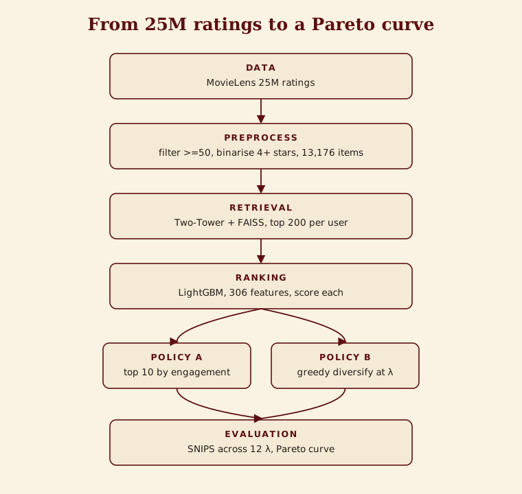
Starting from 25 million ratings, the dataset is filtered to the 13,176 films with at least 50 interactions, and any rating of 4 stars or higher counts as a positive. A Two-Tower model learns 128-dimensional embeddings for those 13,176 films and indexes them in a FAISS IVFFlat index. At request time, the user gets an embedding too, FAISS returns the 200 nearest films, and LightGBM scores each (user, film) pair on 306 features. That gives us the ranked list. Policy A takes the top 10 directly. Policy B runs the greedy reranker on those same scores, picking 10 while penalising genre repetition at strength λ. Running SNIPS evaluation across 12 values of λ traces out the Pareto curve.
Each artifact earns its place. The FAISS index means film embeddings are computed once rather than at every request. A cached test_candidates.parquet, 5,033,200 rows of pre-scored candidates, means the λ sweep never reruns the ranker. It rereads scores and re-sorts. Every stage’s output is the next stage’s checkpoint.
Three things I got wrong
The embedding collapse. I used BatchNorm in the Two-Tower because it is the default move in feedforward tutorials: add normalisation between layers and training stabilises. There was no specific reason to distrust it. What happened instead was two days of training that looked like it was working and wasn’t. The loss fell the whole time. Recall@10 read 0.002, the random-chance floor. I spent too long checking the loss curve and the data loader, because those are usually where problems show up. The actual issue was elsewhere, and it took one specific measurement to surface it.
The embedding collapse, and the diagnostic that caught it
BatchNorm normalises across the batch dimension: for each feature it centres and scales using every sample in the batch. In a classification network that is useful regularisation. In a Two-Tower retrieval model it pushes all the item embeddings in a batch toward a shared distribution, layer after layer, until after about three layers they point in roughly the same direction.
The training loss kept decreasing while Recall@10 read 0.002. When I measured the cosine similarity between each item embedding and the centroid of all of them, it came back 1.000. Every item had become the same vector, so nearest-neighbour search returned arbitrary results because every item was equidistant from every user.
Switching to LayerNorm turns out to fix it because it normalises within each embedding, along its own feature dimension, which leaves different embeddings free to spread out in the space. After the switch, Recall@10 went from 0.002 to 0.147.
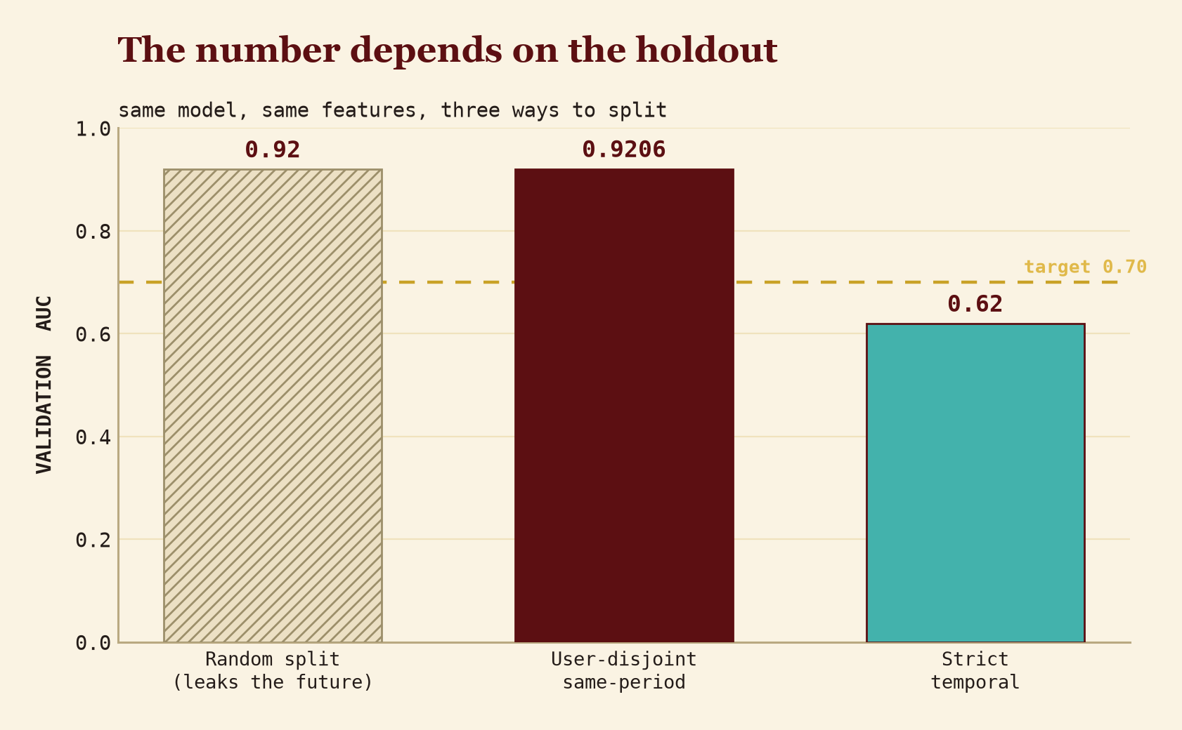
Testing against the future. A random train/test split gave a val_auc of about 0.92. That looked like a good result, but a random split over interaction data leaks: when the same user lands on both sides, with later interactions in training and earlier ones in test, the model has effectively seen future behaviour. The number was inflated.
Switching to a time-respecting holdout, where training uses older data and test uses genuinely newer data, brought the number to about 0.62. The first holdout had been generous with future information. This one is stricter, and 0.62 is the more useful figure for understanding what forward deployment will cost. The two holdouts answer different questions: a user-disjoint, same-period holdout gives val_auc = 0.9206 and measures how well the ranker performs within its training distribution. A strict temporal holdout gives about 0.62 and measures the cost of training on history and serving on future data. Both numbers belong on the record, and any AUC only means something once you know which holdout produced it.
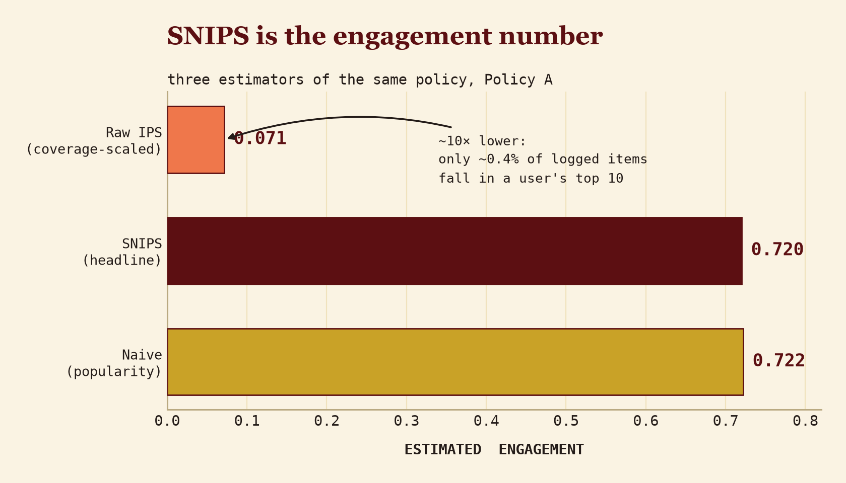
Making sense of the IPS numbers. The first engagement figure I calculated was raw IPS: 0.071. It took a while to understand why that was not the right number to report.
Raw IPS and SNIPS are both estimators of the same underlying quantity, but they treat the denominator differently. Raw IPS divides by the total number of logged events, so it ends up reflecting how much of the interaction log the new policy actually covers. Since only about 0.4% of logged items fall inside a user’s top-10 recommendations, the raw estimate comes out as the in-policy engagement rate scaled down by coverage. Working through the propensities, the self-normalising denominator, and how little of a top-10 list overlaps with any single logged interaction clarified the gap: 0.071 is a coverage-scaled rate, and SNIPS at 0.720 is what actually corresponds to the engagement figure. SNIPS divides by the sum of importance weights instead of the total event count, which cancels the coverage effect. The naive estimator, which skips the propensity correction, comes in at 0.722 for the same policy. Both are estimates of Policy A’s engagement. The near-tie between them says the bias correction is small: a popularity-aligned recommender mostly recommends high-propensity items, so correcting for popularity bias does not move the number much.
Why these tools
Two-Tower with FAISS. A model that scores every (user, item) pair cannot run over the full catalogue at request time. Two-Tower splits the work: item embeddings are precomputed once, the user embedding is computed per request, and similarity search does the rest. I used FAISS IVFFlat rather than HNSW because at 13,176 items the exact-within-cell search is already fast, and HNSW’s graph-construction overhead adds nothing at this size.
LightGBM rather than a neural reranker. The 306 features mix 256 dense embedding dimensions (128 from the user tower, 128 from the item tower), 36 binary genre flags, and 14 scalar features. Trees take that heterogeneity without normalisation, train on roughly 8 million rows in under fifteen minutes, and hand back feature importances for free. A neural reranker would want normalisation, more tuning, and longer training to land in the same place at this scale.
SNIPS rather than raw IPS. Raw IPS is unbiased in theory and high-variance in practice: one item with propensity 0.001 carries an importance weight of 1000 and can swamp the estimate. SNIPS normalises by the sum of importance weights instead of the expected count, trading a little bias for far less variance. Its effective sample size here is 38,280 over 25,166 test users, which says the weights are well behaved and the estimate is worth trusting. Building that machinery, the propensities, the coverage floor, the sample-size check, was where most of the real evaluation work lived.
Why BPR loss instead of cross-entropy
Cross-entropy needs explicit negatives, the items a user disliked. MovieLens only gives positives: a rating of 4 stars or more. An unrated film might just be one the user never saw, so a missing rating tells us little about dislike.
BPR (Bayesian Personalised Ranking) sidesteps that. For each positive it draws a random unobserved item and trains the model to rank the positive higher. Across many samples that is the right signal for implicit feedback, and it never assumes that unobserved means disliked.
One side effect is visible during training: BPR’s Recall@10 oscillates and tends to peak on odd epochs, because the negatives are resampled each epoch. Validating every epoch instead of every second one catches the peaks rather than the troughs.
The trade-offs
Most of these choices come with something on the other side.
Offline against online. SNIPS estimates how a new policy would have done on the same users in the same sessions. It cannot see long-term retention, or what happens when people get more varied recommendations for months. For offline research on a public dataset it is the right tool. The only way to see those longer-term effects is to run the policy on live traffic and watch what real users do over weeks. That is what an A/B test does, and a public dataset cannot provide one, so SNIPS is as far as this project can go.
Same-period against temporal. I kept both holdout numbers on the record on purpose. The same-period holdout (0.9206) measures performance inside the training distribution. The temporal holdout (about 0.62) measures forward deployment. Quoting either one on its own would give a misleading picture of the model.
Pareto against joint training. Because the ranker never sees the diversity objective, a jointly trained model could in principle find a better frontier. What the split buys is legibility: two objectives I can debug separately, and a curve I can hand to someone with “pick a point.” A jointly trained model gives one operating point and cannot show us the shape of the choice.
What generalises
A few of these lessons carry beyond recommender systems.
When a training metric looks healthy and a downstream metric looks poor, the training metric is usually the thing that is wrong. The batch loss was fine while Recall@10 read 0.002. The loss was not lying, it just was not measuring what I cared about. That mismatch shows up in any system where the training objective is a proxy for the real goal, which is most of them.
Keeping the trade-off at inference tends to be more useful than baking it into the weights. The Pareto approach worked here because the diversity decision is applied at inference, where a product manager or an ops team can adjust it without retraining. Any time the people who tune a trade-off are not the people who trained the model, it is worth asking whether the knob can be a runtime parameter instead of a training hyperparameter.
The shape was the surprise
The shape of the curve was what I didn’t expect.
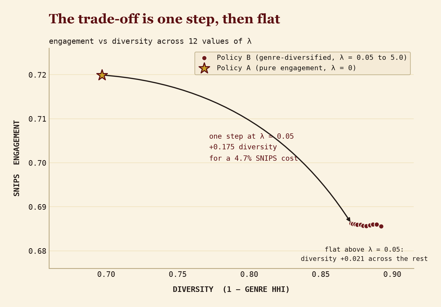
I’d set up the λ sweep assuming a gradient: apply a little diversity penalty, lose a little engagement, proportionally, all the way to λ=5.0. What the results showed instead was a step. At λ=0.05, genre HHI falls from 0.303 to 0.129 and the diversity score climbs from 0.697 to 0.871, while SNIPS slides from 0.720 to 0.686, a 4.7% reduction. Above λ=0.05 the curve flattens: diversity moves another 0.021 across the entire remaining range out to λ=5.0, while SNIPS stays inside a 0.001 band. The whole diversity span across the sweep is 0.195, and almost all of it arrives in that first step.
Looking at the plot, almost everything interesting had already happened by the time λ reached 0.05. The eleven Policy B points above that threshold pile into a tight cluster in the upper right of the chart. Pushing harder on λ barely moves the curve.
That changes what we’re deciding. “Find the optimal λ” turns out to be the wrong frame. The choice is closer to binary: take the step at λ=0.05, or stay at Policy A. Once we do, any λ above 0.05 lands in roughly the same flat region, so the exact value matters very little. What varies within it is how much we value showing people things outside their usual cluster, and that is not something the Pareto curve can answer for us.
A jointly trained loss would have averaged this structure away: a fixed λ in the training objective would give one point on the frontier, with no way to see that almost all of the achievable diversity is concentrated in a single transition. The step is only visible because the diversity penalty is kept separate from training and applied at inference.
The full build, including the per-phase docs and the deviation log this post draws on, is in the project repo.