11 Jun 2026 · 4 min read
Feature Importance Stability in AutoML Forecasting
How SHAP feature rankings compare across near-optimal models, within a training window and as it moves forward in time.
Question
SHAP (SHapley Additive exPlanations) is a method that assigns each feature a contribution to a single prediction: how much the most recent reading pushed a forecast up, how much the hour of day pulled it down. It produces one such set of contributions per model. But for most forecasting problems there are lots of models that score about the same. The Rashomon set is the name for that crowd, after the film in which several witnesses give different accounts of one event: every model that fits nearly as well as the best one. The models score almost the same on accuracy. They can still rank different inputs as most important.
This disagreement matters for explanation. Forecasting problems like these are increasingly solved with AutoML: automated machine learning systems that train many candidate models and pick the best by an accuracy measure, with no person choosing the model directly. If two equally accurate models produce different accounts, then explaining the single model an AutoML system ranks first describes that model, and may not describe the data behind it. This is from my Masters’ thesis: six forecasting benchmarks run through two AutoML systems. I examined whether the near-optimal models ranked the same inputs as most important, within a single training window, and whether the combined ranking persists as the window advances through time.
Setup
I built the Rashomon set by taking the lowest-error model and keeping every model within a factor of (1 + ε) of it, at five tolerances from 0.02 to 0.30, so ε = 0.05 keeps every model within 5% of the best one’s error. I built it with two AutoML frameworks, since the way models are searched may affect the answer. AutoGluon on its best quality preset builds most of its models from one family through bagging (training many versions of a model on resampled data and averaging them) and a stacking layer (a further model that combines their outputs). H2O AutoML trains a grid over gradient-boosted trees, random forests, extremely randomised trees, and a linear model. I ran both on six forecasting benchmarks, including the ETT family and M4 Monthly, with three random seeds each and rolling-origin splits so that no future information enters the training window.
For each set I computed SHAP importances and compared the feature rankings with the Spearman rank correlation, a measure of how similarly two models order the same features. It takes values from -1 to 1: at 1 the two rankings are identical, at 0 they have no relationship. I made the comparison two ways, within a single window and across consecutive windows.
Agreement within a single window
The near-optimal models ranked features in a similar order within a training window. Across both frameworks, on every benchmark where more than one model qualified, mean pairwise Spearman ranged from 0.664 to 0.989, with the lowest correlation on the Cable Demand benchmark.
Agreement across time
The combined ranking also persisted as the window advanced.
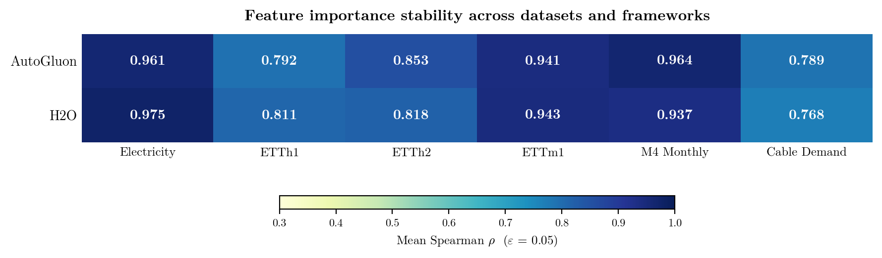
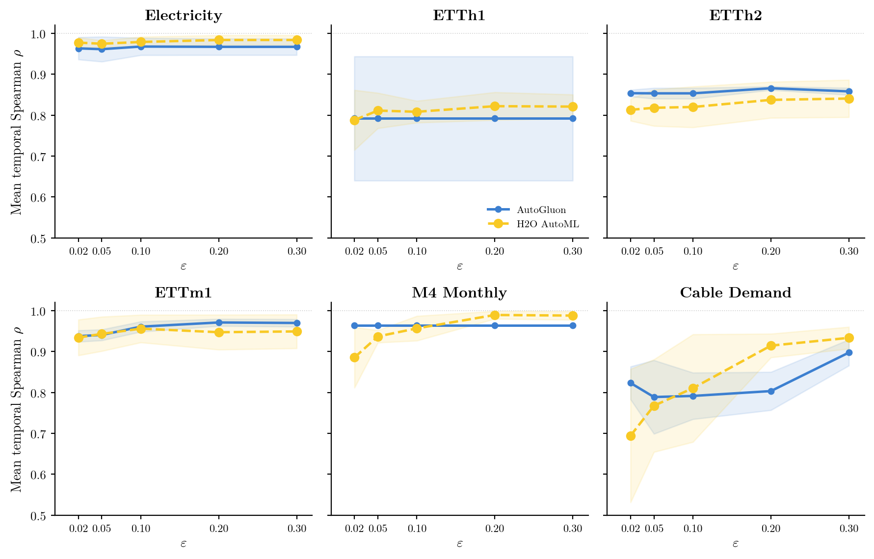
Mean temporal Spearman ranged from 0.768 to 0.975 across the twelve benchmark and framework pairs, and the two frameworks were comparable on every benchmark. Agreement persisted as ε widened, including at the tolerance where an additional model family entered the set.
How the models are combined
Combining a set of models into one ranking requires a choice that affects the result. I ranked each model’s features first, then averaged those ranks. The alternative averages the raw SHAP magnitudes across models. A single model with much larger values can then determine the average.
H2O’s random forest and extremely randomised trees models are explained with a fast approximation (Saabas) rather than the exact method, and this approximation’s values can be many orders of magnitude larger than the exact method’s. On the electricity benchmark, averaging the raw magnitudes reduced the combined ranking’s temporal correlation to near zero, at the tolerance where such a model first qualified. Averaging ranks instead removes this scale inflation, and the same comparison stays above 0.95. The instability measured under magnitude averaging is a property of the aggregation rather than of the models. Restricting the within-window comparison to models with exact SHAP raises agreement on that benchmark by about 0.09, consistent with the approximation changing the order of that model’s own features.
What the framework contributes
The two frameworks produced sets of different size and composition. AutoGluon produced a single model on four of the six benchmarks at the narrowest tolerance, and small sets on the rest. AutoGluon builds most of its models from one family through bagging and a stacking layer, so that family’s error is well below the others and few other models qualify. H2O produced larger and more varied sets, up to its training budget of about 20 models.
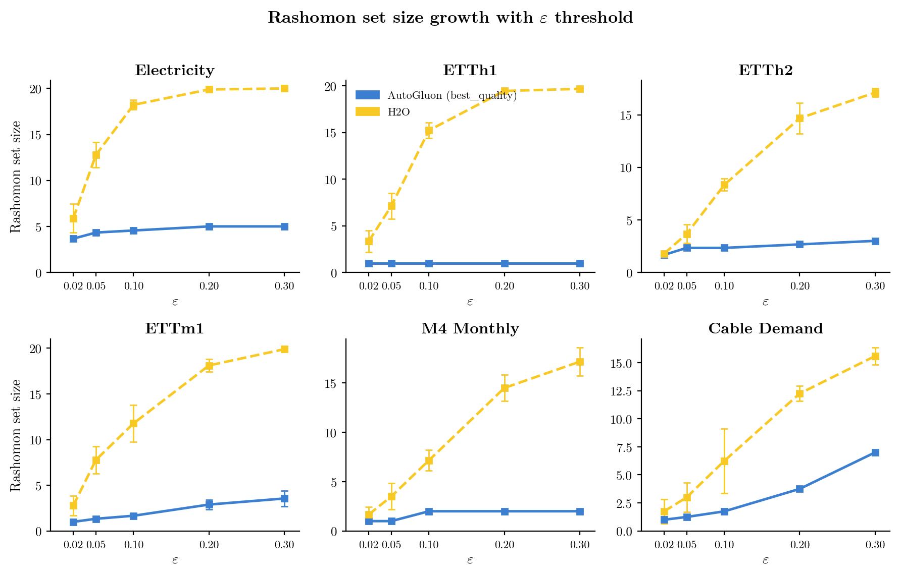
Rank agreement was comparable across both, so the greater size and variety of the H2O sets did not lower stability.
What it suggests
The results suggest that an explanation of a single near-optimal model is more dependable once it has been shown to persist across the near-optimal models and across successive training windows. Across these six benchmarks, rankings were more stable where a few features carried most of the importance, and less stable where importance was spread across many, an association observed under both frameworks.
The code is on GitHub, where the full thesis will follow.